Conditional formatting is useful in highlighting values for certain conditions / criteria to easily identify trends.
There are predefined formatting options already added for you from simply selecting the range you would like to apply formatting and within the Home Ribbon in the Styles group is the following:

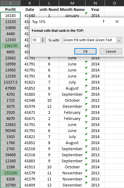
You can simply select one of these options. Here we’ve selected the range of profit data and selected Top/Bottom Rules and selected Top 10%. The percentage range can be changed along with the formatting style used to highlight the values that hit the selected criteria.

Custom Conditional Formatting Rules
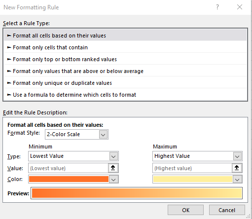
To create more complex conditional formatting rules back within conditional formatting there is an option to create a New Rule but also Manage Rules that we have created in the workbook.

Here there are a variety of options for rule types. The most common option is Use a formula to determine which cells to format