There are a multitude of excel functions that can help complete analysis, filtering, checking, sorting, returning etc data. There are so many that not all of them are described here.
These are some of the most common functions that are very handy with completing the tasks just mentioned, but there are also math, text, statistic, logic, engineering, financial and date/time functions that aren’t listed here.
The functions here are used often and have dynamic uses within excel hence they are chosen to help improve efficiency when working with data.
The examples shown are kept simple to help grasp the high level functionality of the functions to be able to adapt to your data set.
Simple Functions
IF Function
The Excel IF function is a logic test which either returns a True OR FALSE result.
This function is perfect to filter results, check data, complete different formulas depending on results and also be able to be nested to test for a variety of conditions.It’s probably one of Excels most popular functions.
Syntax for IF Functions:
The function follows the following logic:
=IF(logic_test,[value_if_true],[value_if_false])
Example 1
Let’s start with with a simple Yes or No result for if students pass their assessment here we use =IF(A2>0.5,"Yes","No") since the data in the column A is in decimal values shown in the percentage number format, where 0.5 is 50%.
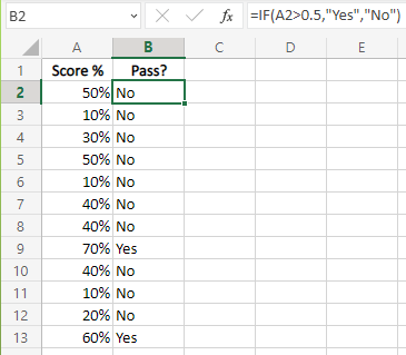
For this example the returned value is text defined by " ", but we could have this as anything we want, so something like =IF(A2>0.5,"Pass","Fail") could also be used here.
We also use the logic operator > which means greater than but we can also use different operators.
| Logic Operator | Meaning |
|---|---|
| = | Equal to |
| < | Less than |
| > | Greater than |
| <= | Less than or equal to |
| >= | Greater than or equal to |
| <> | not equal to |
Example 2
Now we can also complete formulas depending on the logic test. Say we measure temperature before and after and we only want to take the temperature change if it was recorded.
Using =IF(E3<>0,D3-E3,"No End Recorded") if the End Temperature Column doesn’t equal 0, then calculate the difference otherwise return No End Recorded text.
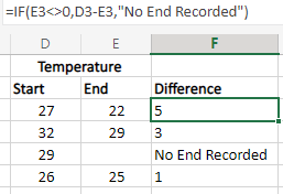
This examples shows the use of formulas as the true result and a text result for the false result.
Example 3
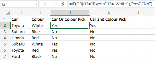
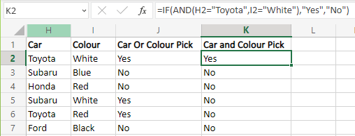
The IF Function can also be combined with the AND/OR criteria. This introduces multiple criteria to the IF Function.
In this example we want a White Toyota, where in column J we assign the pick if the car is either a Toyota OR White, whereas in column K we assign the pick if the car is both White AND a Toyota.
IFS Function
The IF Function can be nested to capture multiple criteria, but this can be difficult where there are several criteria.
To complete the same purpose the IFS Function can be used which follows the following logic:
=IFS(logic_test1,value_if_true_1,...)
Example 3
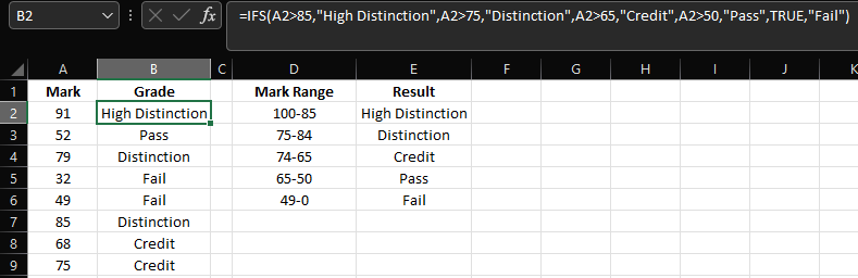
This example uses multiple criteria to give resulting grades over certain mark ranges. Where if the logic test doesn’t fall within the range then a Fail grade is given.
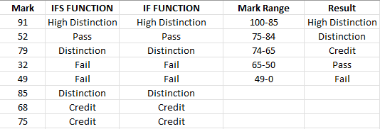
As mentioned before a nested IF Function can also be used:
=IF(A2>85,"High Distinction",IF(A2>75,"Distinction",IF(A2>65,"Credit",IF(A2>50,"Pass","Fail"))))
Whilst the IFS Function used is:
=IFS(A2>85,"High Distinction",A2>75,"Distinction",A2>65,"Credit",A2>50,"Pass",TRUE,"Fail")
The formula for both are about the same length, but keeping track of brackets and commas can lead to easy formula errors.
Both results from both the IFS and IF Function are put side on.
SUM Function
The SUM Function results the total of a range of numbers using:
=SUM(number1, number2, ...)
Completing this function can also be done automatically using AutoSum in the Home Ribbon within the Editing group.
Just select the cell at the bottom of th values and it will sum the column.
Example 4
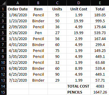
In this example selecting E14 and clicking the AutoSum command will sum the Total column E similarly this can be completing using the formula =SUM(E2:E13)
SUMIF Function
In Example 4 the total cost of Pencils are calculated using the SUMIF Function which is similar to the previous function IFS statement previously mentioned. The SUMIF Function follows the logic below:
=SUMIF(range, criteria, [sum range])
where for Example 4 the formula in cell E15 is:
=SUMIF(B2:B13,"Pencil",E2:E13)
SUMIFS Function
This function is again similar to the SUMIF Function but where:
=SUMIFS(sum_range, criteria_range1, criteria1, criteria_range2, criteria 2, ...)
Which is much more useful when dealing with multiple criteria and ranges.
COUNT Functions
There are multiple count functions which can be useful depending on the type of data or filtering you require.
//incrementally adds to the count for the set values selected or over a range
=COUNT(value1, value2, ...)
//only adds to the count if the set criteria is TRUE
=COUNTIF(range, criteria)
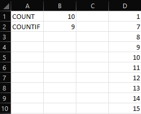
Example 5
Here we see both functions and their results. The function for COUNT uses =COUNT($D$1:$D$10), where the function COUNTIF uses =COUNTIF($D$1:$D$10,">5") where the function is only adding to the count IF the value in column D is > 5 therefore the result is 9 instead of 10.
Versatile Functions
INDEX Function
The syntax of the index function is:
=INDEX(array, row_num, [column_num])
Where the function will return the value of an element within the array that corresponds to the row and column number indexes entered.
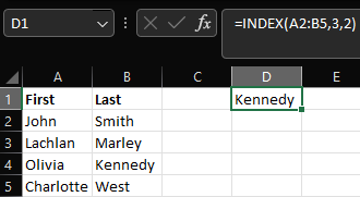
Example 6
The formula here is =INDEX(A2:B5,3,2) where it returns the 3rd row in the second column in reference to the array range.
This results with the Last name of “Olivia Kennedy”.
Another syntax of the Index function is the use of areas when having multiple array sections where:
=INDEX(reference, row_num, [column_num], [area_num])
Example 7
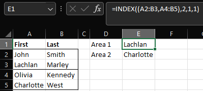
Using the same data in Example 6 but splitting the array into two sections where:
- Area 1: Male Names
- Area 2: Female Names
For both results were selecting the 2nd row in the first column where Area 1 uses index 1 and Area 2 uses index 2 for the [area_num] part of the function.
| Area Index | Meaning |
|---|---|
| 1 | =INDEX((A2:B3,A4:B5),2,1,1) |
| 2 | =INDEX((A2:B3,A4:B5),2,1,2) |
Entire Rows / Columns
The Index function is very versatile as it can be adapted to return entire rows =INDEX(range,1,0) or columns =INDEX(range,0,n)
MATCH Function
The Index function follows the syntax:
=MATCH(lookup_value, lookup_array, [match_type])
The lookup_value will be the value you’d like to match with, lookup_array is the range of where to look for this value and the match_type which has the options of (1, 0, -1) which correspond to [less than, exact, greater than]
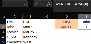
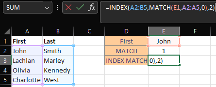
Example 8
Here to look for the First name John by taking the cell reference E1 and looking for the match in the range A2:A5
Nesting MATCH Function with INDEX
The Match function can be nested within the Index function to return a row number and or a column number when a match is found.
Example 9
For this first example the match function is used to return the row number to match the first name John then return the 2nd column resulting in returning John’s last name which is Smith.
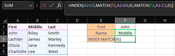
Example 10
Adding a middle name to the data set can show using both the match function within the index function for both the row number and the column number.
Here the first name is matched with the selection of John for the row number, then for the column for which name should be return is the middle name which gives Riley.
VLOOKUP Function
This function is similar to nesting the match function inside an index function, but with this function the lookup value must be in the first column where the function uses the following syntax:
=VLOOKUP(lookup_value, table_array, col_index_num,[range_lookup])
The Vlookup function stands for vertical lookup where the row is the looking index.
The range_lookup has the options of (True, False) which corresponds to either (approximate match, exact match)
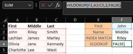
Example 11
Similar to Example 10 the same result can be created with the lookup function with:
=VLOOKUP(F1,A2:C5,2,FALSE)
Here the lookup value is the first name over the same range returning the second column which is the middle name with an exact match with FALSE.
HLOOKUP Function
This function performs the same as the Vlookup function but stands for horizontal lookup but now the column is the looking index.
The syntax is the following:
//The lookup value must be in the first row of the table
=HLOOKUP(lookup_value, table_array, row_index_num, [range_lookup])
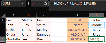
Example 12
To return the same value as Example 11 the lookup value is now the middle name and the defined row number in the array is 2 for John’s middle name using an exact match with FALSE.
XLOOKUP Function
Following through the examples it can be seen that there are limitations to lookups depending on the setup of the dataset, this is why nesting match functions within an index function can be handy as it can specify the row or column index without being in the first row or first column.
This is where the Xlookup function can be handy as the returned results don’t have to be on a specific side of the lookup index.
The function follows the following syntax:
=XLOOKUP(lookup_value, lookup_array, return_array, [if_not_found], [match_mode], [search_mode])
This function has optional arguments:
- [if_not_found] when a match isn’t found a defined returned value or text can be defined instead of returning
#N/A - [match_mode] specifies the match type with the options of (1, 0, -1, 2) which corresponds to
(exact match, exact match if none then next smaller item, exact match if none then next larger item, wildcard match(*,?,~)) - [search_mode] specifies the search type with the options of (1,-1, 2, -2) which corresponds to
(ascending search, reverse search, ascending binary, descending binary)
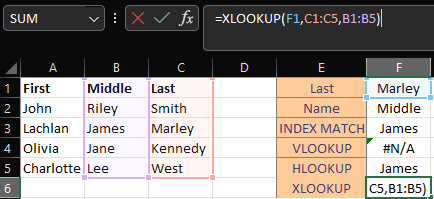
Example 13
For this example to show the limitations of the functions that are mentioned the lookup value with now be the last name of Lachlan and return the middle name.
For the Xlookup function the return value is on the left hand side of the lookup value which is ok for this function as it doesn’t matter. Therefore the returned middle name is James
But as you can see the Vlookup value returns an error #N/A this is because the return value is to the left of the lookup value which the function doesn’t allow.
The Hlookup can find the value as the lookup value is the column which is still the first row and for the index match it doesn’t matter as the lookup arrays are defined for each match value.